SQL has come a long way since it was first introduced in the 1970s. As of 2026, there are now over 160 relational databases (according to DB-Engines), with SQL being the third most popular language used by developers (according to the 2025 Stack Overflow Developer Survey).
We’ve seen 10 iterations of the SQL standard, but many of the relational database systems have implemented a huge variety of vendor-specific features in their SQL language.
Given how broad “SQL” is as a topic, our upcoming articles highlight some of the modern SQL features that we’ve come to love — and we’re sure that you’ll love, too!
Table of content
- Filter results with QUALIFY
- RANGE and GROUPS in windows
- EXCLUDE rows in a window frame
- NULL-safe comparison with IS [NOT] DISTINCT FROM
- Expressive join types
- Transpose tables with PIVOT and UNPIVOT (coming up in part 2)
- Advanced GROUP BY options (coming up in part 2)
- Simplified grouping with GROUP BY ALL (coming up in part 2)
- First-class support for compound data types (coming up in part 2)
- Recursive common table expressions (coming up in part 2)
This article starts with the first 5. Stay tuned for the second article covering the rest of the list!
1. Filter results with QUALIFY
This is easily one of the most popular clauses in modern SQL. The best way to think of QUALIFY is that QUALIFY is the window equivalent of HAVING. This means that a SQL query now has three places that it can apply filters (excluding inner joins):
WHERE: filters rows before any joins and calculationsHAVING: filters rows immediately after any aggregationsQUALIFY: filters rows immediately after any window expressions
A common pattern prior to QUALIFY was to use a window function in a CTE/subquery and filter on its result in a downstream WHERE clause. The QUALIFY clause means that we don’t need the CTE/subquery! For example, selecting the most recently updated customer records:
Without QUALIFY
|
With QUALIFY
|
Using QUALIFY is much cleaner!
The QUALIFY clause is available in many modern data platforms, such as:
2. RANGE and GROUPS in windows (not just ROWS!)
If you’ve ever bounded a window range, chances are you’ve only ever really used the ROWS frame type. For example, calculating a 7-day running total of sales:
select
  sales_date,
  sum(revenue) over (
	  order by sales_date
	  rows between 6 preceding and current row
	) as seven_day_running_total
from sales
The ROWS frame type is intuitive, but it’s not always the most appropriate frame type to use. There are two more frame types, RANGE and GROUPS; simplified definitions of all three are:
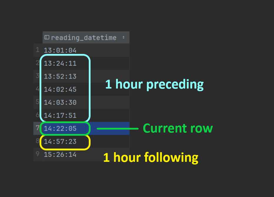
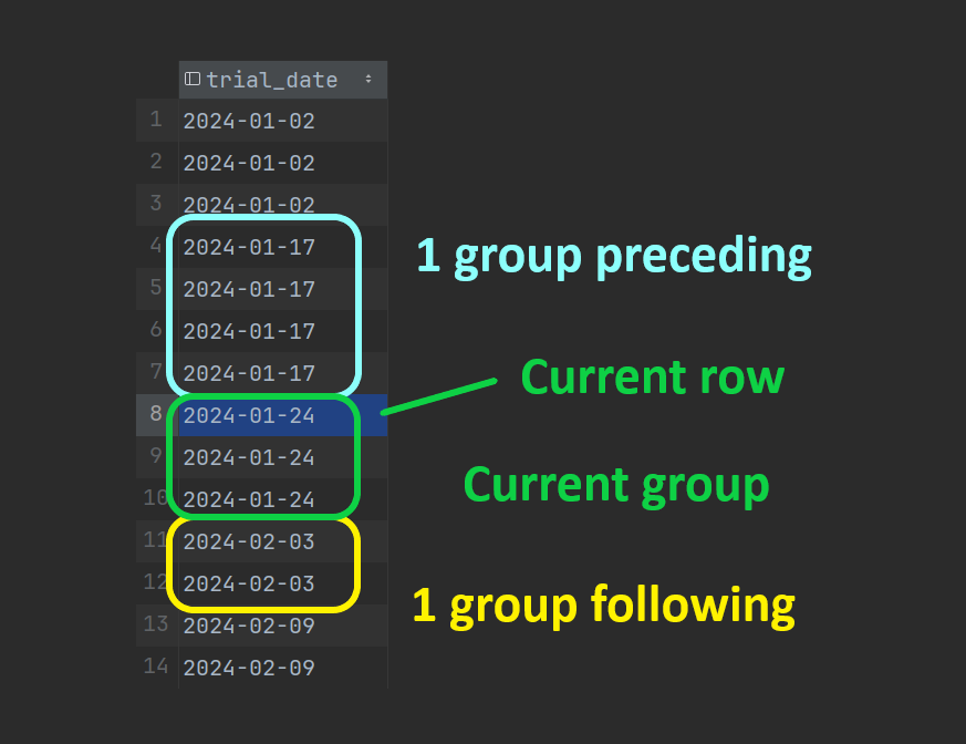
ROWSkeeps surrounding rows by how many rows away they are from the current rowRANGEkeeps surrounding rows by their value difference relative to the current rowGROUPSkeeps surrounding rows by how many distinct values away they are from the current row
To help illustrate how RANGE and GROUPS work, the images below highlight which rows would be included in some example queries (DuckDB/PostgreSQL compatible syntax):
RANGE query
select
  reading_datetime,
  temperature,
  avg(temperature) over (
    order by reading_datetime
    range between interval '1 hour' preceding
              and interval '1 hour' following
  ) as avg_temperature_within_hour
from readings
RANGE selected rows
GROUPS query
select
  trial_date,
  sum(trial_result = 'succeed') over running_trials as succeeded,
  sum(trial_result = 'fail')    over running_trials as failed
from trials
window running_trials as (
  order by trial_date
  groups unbounded preceding
)
order by trial_date
GROUPS selected rows
RANGE is a frame type that we like to use, but GROUPS is almost never needed so many database engines don’t even support it.
| Database | Supports RANGE |
Supports GROUPS |
|---|---|---|
| Snowflake | ✅ | ❌ |
| Databricks | ✅ | ❌ |
| BigQuery | ✅ | ❌ |
| SQL Server | ✅ | ❌ |
| ClickHouse | ✅ | ❌ |
| DuckDB | ✅ | ✅ |
| PostgreSQL | ✅ | ✅ |
| SQLite | ✅ | ✅ |
3. EXCLUDE rows in a window frame
Using ROWS/RANGE/GROUPS is great for adding more rows to the window frame, but it’s not uncommon to want to also exclude some rows from the frame.
A few databases support the EXCLUDE option at the end of a window frame precisely for this:
... OVER (
    PARTITION BY ...
    ORDER BY ...
    ROWS | RANGE | GROUPS ...
    EXCLUDE ...
)
There are four options for EXCLUDE: NO OTHERS, CURRENT ROW, GROUP, and TIES. The SQLite and PostgreSQL docs do a good job of describing these, which we summarise below. Note that the “peers” of a row are the rows in the same partition that have the same ordering value.
NO OTHERS: The default behaviour — don’t exclude anythingCURRENT ROW: Exclude the current rowGROUP: Exclude the current group (the current row and its peers)TIES: Exclude the row’s peers, but not the current row
For example, if you’re doing anomaly detection, you may want to compare the current row’s value to the average of the values around it: using EXCLUDE CURRENT ROW would allow you to do that in a single window!
select
  reading_datetime,
  temperature,
  avg(temperature) over (
    order by reading_datetime
    range between interval '1 hour' preceding
              and interval '1 hour' following
          exclude current row
  ) as avg_temperature_within_hour_excluding_current_row
from readings
The EXCLUDE option is available in only a handful of databases, including:
4. NULL-safe comparison with IS [NOT] DISTINCT FROM
NULL is the gift that keeps on giving when it comes to bugs in SQL queries.
We all know that we should use = for comparing two non-null values, and IS [NOT] for comparing a nullable value to NULL, but comparing two nullable values has always been a bit fiddly: first check whether they’re both NULL, then whether either are NULL, then finally do the = comparison.
There are some concise implementations, but they’re mostly unintuitive when you first encounter them.
A better alternative is the NULL-safe operator IS [NOT] DISTINCT FROM. This operator will treat NULL as a known value, which leads to far more intuitive results. For example:
1 IS DISTINCT FROM 2→ true1 IS DISTINCT FROM NULL→ trueNULL IS DISTINCT FROM NULL→ falseNULL IS NOT DISTINCT FROM NULL→ true1 IS NOT DISTINCT FROM NULL→ false
It’s a bit more wordy, but using this operator for nullable columns is considerably safer than using just =, and this operator is a better alternative to explicit NULL handling.
Old NULL-safe comparison logic
case
  when val_1 is null and val_2 is null
    then false
  when val_1 is null or val_2 is null
    then true
    else val_1 != val_2
end as is_different
New NULL-safe comparison
val_1 is distinct from val_2 as is_different
The IS [NOT] DISTINCT FROM operator is part of the SQL standard (from SQL-2023) and is supported in most databases.
5. Expressive join types (SEMI/ANTI, ASOF, LATERAL)
We’ve come a long way since the SQL-92 joins!
The 1992 SQL standard introduced the joins that we’re all familiar with:
CROSSINNERLEFT [OUTER](andRIGHT [OUTER])FULL [OUTER]
Over thirty years later, we’ve found ourselves needing some more expressive joins — particularly in the OLAP world. The implementation of these expressive join types can differ between databases (if they’re supported at all), so make sure you check the docs for your database if you want to use some of these!
SEMI and ANTI joins
The term “semi-join” and “anti-join” have been used for a long time, and have historically been in reference to using a WHERE condition to filter rows based on their existence in another table. Specifically:
- A “semi-join” will keep rows in the base table if their values exist in the referenced table
- An “anti-join” will remove rows in the base table if their values exist in the referenced table
For example, the queries below are both a “semi-join” which keeps customer records for customers that have a “login” event:
select *
from customers
where customer_id in (
  select customer_id
  from events
  where event_name = 'login'
)
select *
from customers
where exists(
  select *
  from events
  where customers.customer_id = events.customer_id
    and event_name = 'login'
)
Even though we don’t use the JOIN keyword, we still refer to these as “joins” — and it’s easier to see why in the subquery example on the right.
That said, some databases have explicitly implemented SEMI and ANTI as join types, which would allow the following modern SQL that’s equivalent to the queries above:
select *
from customers
  semi join events
    on customers.customer_id = events.customer_id
    and events.event_name = 'login'
ASOF joins
A common join requirement is “match the record with the same ID that’s the closest to a given timestamp”, commonly referred to as an “as-of” join. For example, matching a financial transaction to the most recent currency exchange rate relative to the transaction time.
Snowflake, ClickHouse, and DuckDB have each implemented this as an explicit ASOF join, but all three have a slightly different syntax for it!
Below is a Snowflake example and a DuckDB example for joining transactional data to exchange rate data using an “as-of” join:
/* Snowflake */
select
  transactions.*,
  exchange_rates.rate
from transactions
  asof join exchange_rates
    match_condition (transactions.transaction_ts >= exchange_rates.valid_from)
    on transactions.currency_code = exchange_rates.currency_code
    and exchange_rates.to_currency = 'GBP'
;

/* DuckDB */
select
  transactions.*,
  exchange_rates.rate
from transactions
  asof left join exchange_rates
    on transactions.currency_code = exchange_rates.currency_code
    and exchange_rates.to_currency = 'GBP'
    and transactions.transaction_ts >= exchange_rates.valid_from
;
If your database doesn’t support these “as-of”, it’s common to use either a lateral join, or a “normal” join which then filters for the closest row using a window function.
Lateral joins
A “lateral join” is just a join on a correlated subquery!*
These aren’t needed very often, but (where supported) they offer a huge amount of flexibility compared to traditional joins. However, they can also come at the cost of significantly degraded performance, so use these with caution.
In most databases that support lateral joins, there are generally two ways they’re written:
select ...
from ...
	cross join lateral (
	  <correlated subquery>
	)
select ...
from ...
	left join lateral (
	  <correlated subquery>
	) on true
Note that, for the LEFT JOIN version, there is often no join condition outside of the correlated subquery (including it in the subquery is what makes it correlated!), but you can still include additional conditions on the outside if you want — where the database supports it.
Also note that LATERAL isn’t an explicit join type: it’s a keyword specified after JOIN to indicate that the following subquery will be correlated. The CROSS JOIN version acts like an inner join by dropping rows that don’t have a result in the correlated subquery, while the LEFT JOIN version keeps the unmatched rows.
SQL Server also implements lateral joins, but not using the LATERAL keyword — instead, it has the APPLY operator with CROSS and OUTER variants corresponding to the CROSS and LEFT join variants above:
select ...
from ...
	cross apply (
	  <correlated subquery>
	) as t
select ...
from ...
	outer apply (
	  <correlated subquery>
	) as t
We mentioned a practical usage for lateral join above: implementing an “as-of” join in a database that doesn’t explicitly support the ASOF join type. You can find examples of this HERE.
*There’s some nuance around what counts as a lateral join. In this article, we just consider lateral joins as joining on correlated subqueries.
However, some databases also support a more generalised lateral join which supports joining on (a transformation of) a column in the base table, mainly for unpacking nested values in the column.
We won’t cover these generalised joins here, but examples include:
| Database | Explicit SEMI/ANTI | ASOF | LATERAL |
|---|---|---|---|
| Snowflake | ❌ | ✅ | ✅ (limited) |
| Databricks | ❌ | ❌ | ✅ |
| BigQuery | ❌ | ❌ | ❌ |
| SQL Server | ❌ | ❌ | ✅ (APPLY) |
| ClickHouse | ✅ | ✅ | ❌ |
| DuckDB | ✅ | ✅ | ✅ |
| PostgreSQL | ❌ | ❌ | ✅ |
| SQLite | ❌ | ❌ | ❌ |
One of the Tasman folk has a YouTube series on some of these expressive join types: Bill Wallis: Everything about joints.
Stay tuned for part 2!
The features we’ve covered represent just the beginning of modern SQL’s capabilities. Just as modern data teams are adopting faster development tools across the stack, SQL continues evolving to meet contemporary analytical needs. In Part 2, we’ll explore advanced ways of aggregating data, support for compound data types, and the mysterious recursive CTEs.